This is a demo post to explore different optimisation algorithms. To increase understanding I would use a small elliptic 2D cost funtion. Code implementation for all optimizers used in this blog can be found in the github repo
Setting up code
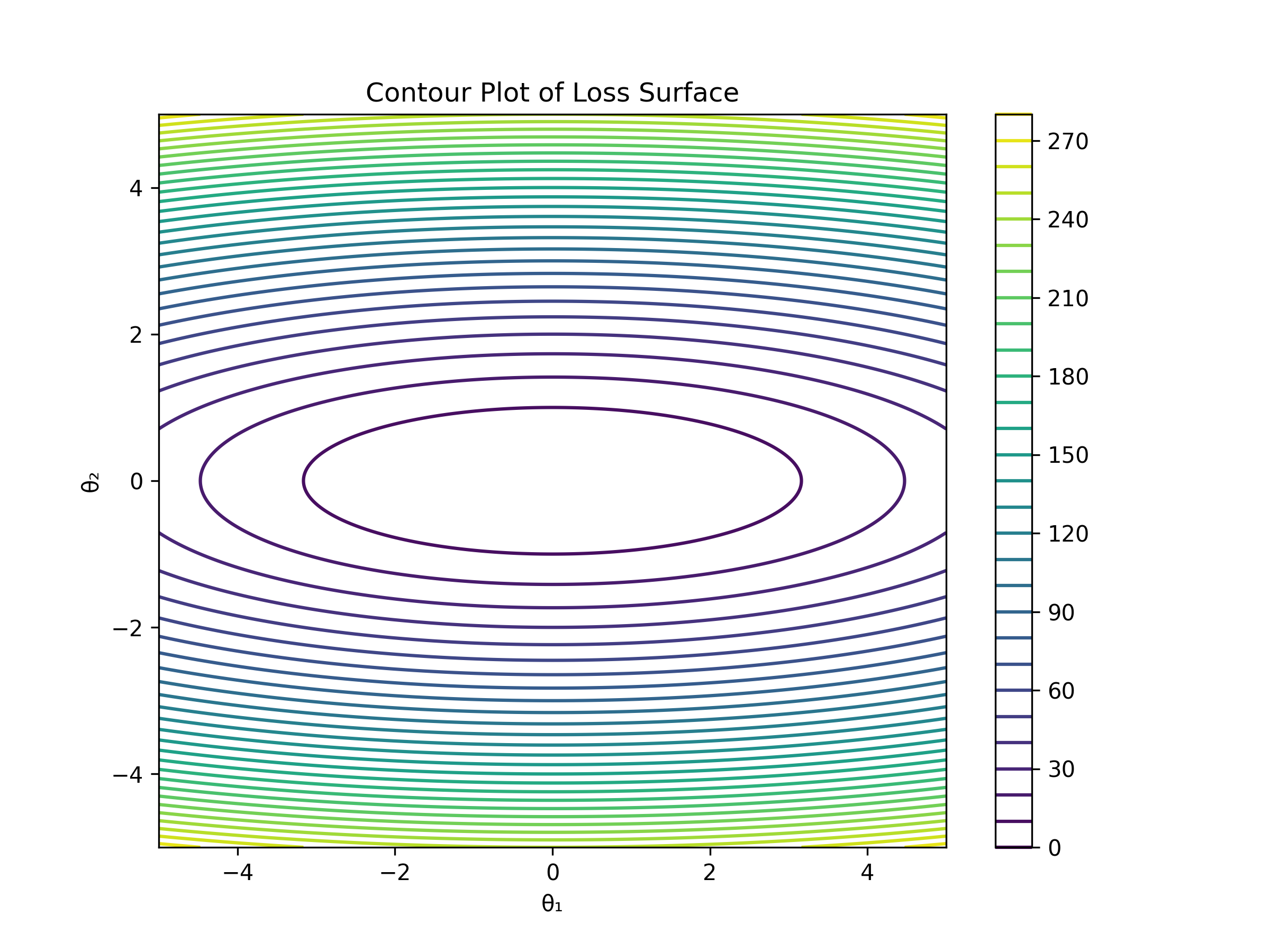
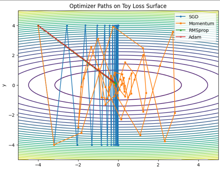
def loss_fn(x, y):
    return x**2 + 10 * y**2

def grad_fn(x, y):
    return np.array([2 * x, 20 * y])

x_vals = np.linspace(-5, 5, 400)
y_vals = np.linspace(-5, 5, 400)
X, Y = np.meshgrid(x_vals, y_vals)
Z = loss_fn(X, Y)
Our loss surface looks like this :
Optimizers
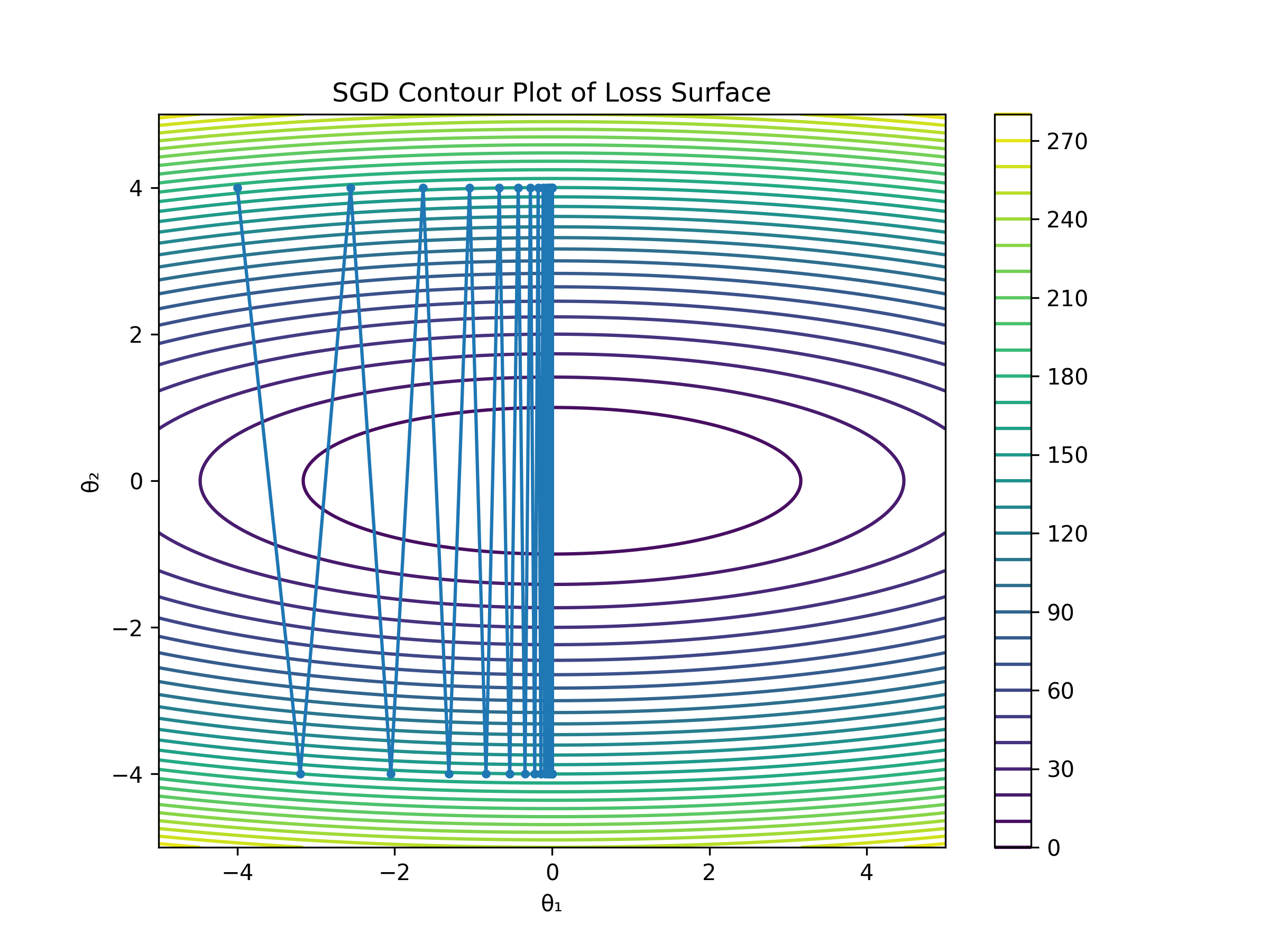
1. SGD
Updates params using gradient of the loss function .
\[\theta_{t+1} = \theta_t - \eta \cdot \nabla J(\theta_t)\]where:
- \( \theta_t \): parameters at step \( t \)
- \( \eta \): learning rate
- \( \nabla J(\theta_t) \): gradient of the loss
The basic idea is to move in the direction of steepest descent and repeat the process from the new position, iteratively. It’s easy to implement, but it can be noisy—especially on mini-batches or high-variance gradients, as we can see in the plot below.
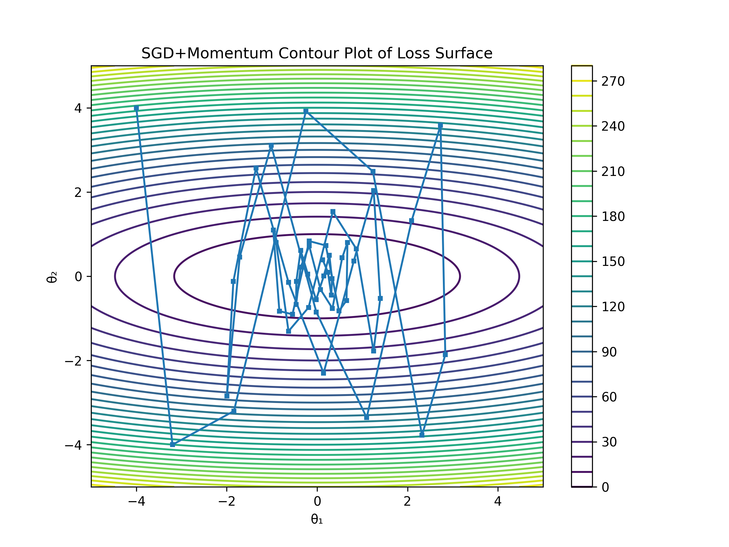
2. SGD with Momentum
Momentum is an extension of SGD that accumulates a moving average of past gradients to smooth out the update path.
This normally results in faster convergence and less oscillation
\[v_t = \beta \cdot v_{t-1} + (1 - \beta) \cdot \nabla J(\theta_t) \\ \theta_{t+1} = \theta_t - \eta \cdot v_t\]where:
- \( \beta \): momentum coefficient
Momentum intution
momentum intuition : I think of them as two vectors , past & present gradients , past gradients influence where resultant gradient vector will go now.
Difference between momentum SGD & SGD
- SGD: Each step is based solely on the current gradient
- Momentum: Combines the current gradient with the previous “velocity” (past gradients), giving updates a sense of direction
3. NAG
Similar to Momentum but looks ahead while computing the direction of change
\[v_t = \beta \cdot v_{t-1} + (1 - \beta) \cdot \nabla J(**\theta_t - \eta \cdot \beta \cdot v_{t-1}**) \\ \theta_{t+1} = \theta_t - \eta \cdot v_t\]where:
- \( \beta \): momentum coefficient
- \( \theta_t \): model parameters
- \( v_t \): velocity (momentum term)
- \( \eta \): learning rate
- \( \nabla J(\cdot) \): gradient of the loss function
- \( \theta_t - \eta \cdot \beta \cdot v_{t-1} \): lookahead position — NAG computes the gradient at this anticipated point instead of the current position
NAG intution
NAG intuition : unlike momentum, which uses the current gradient, NAG “peeks ahead” by first moving in the direction of the previous velocity and then correcting based on the gradient at that lookahead position.
4. Adagrad
It adapts the learning rate for each parameter individually based on its pasr gradients. Parameters that receive frequent updates get smaller learning rates, while infrequently updated ones get larger learning rates.
\[G_{t,i} = \sum_{\tau=1}^{t} g_{\tau,i}^2\] \[\theta_{t+1,i} = \theta_{t,i} - \frac{\eta}{\sqrt{G_{t,i} + \epsilon}} \cdot g_{t,i}\]where:
- \( \theta_{t,i} \): value of parameter \( i\) at time \( t \)
- \( g_{t,i} \): gradient of loss w.r.t. \( \theta_{i} \) at time \( t \)
- \( G_{t,i} \): sum of squares of gradients for parameter \( i \) till time \(t\)
- \( \eta \): initial learning rate
Intuition
- Frequent features get smaller learning rates over time as gradients accumulate over time
- Rare features get larger learning rates
- An important thing to note here : past 3 algorithms were directional in nature , this one focuses on adaptive learning rate ( per parameter )
Issue
Because Adagrad keeps accumulating squared gradients in ( G_{t,i} ), the denominator keeps growing, which can lead to learning rates decreasing too much — eventually stopping updates. Later optimizers like RMSprop and Adam improve upon this.
5. RMSprop
RMSprop resolves Adagrad’s diminishing learning rate by doing exponential moving average limiting the accumulation of squared gradients . It also effectively Denoises gradient

where :
- \( \gamma \): decay rate
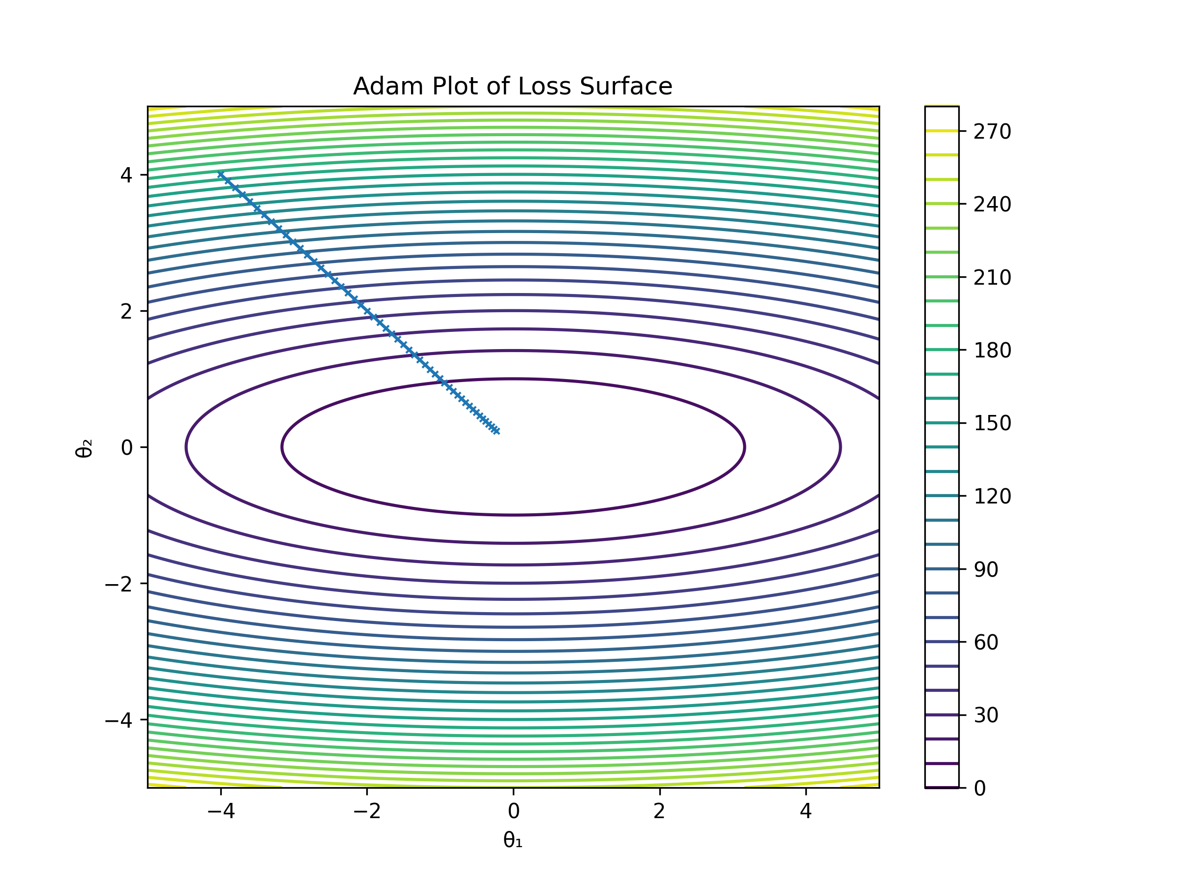
6. Adam
If you noticed, both Adagrad and RMSProp improve learning rates adaptively, but neither uses momentum. Adam combines the benefits of Momentum (smoother convergence) and RMSProp (adaptive learning rates) into one powerful optimizer.
Working of Adam Algo
Adam maintains two moving averages:
- \( m_t \): First moment estimate (~ momentum) :Exponentially decaying average of past gradients
- ( v_t ): Second moment estimate (~ RMSprop) : Exponentially decaying average of squared gradients (like RMSprop)
Both 1st & 2nd moment estimates are biased toward 0, especially during the early steps. At start, \( m_t \) and \( v_t \) are close to 0 due. Without correction, they would underestimate the true mean and variance. Dividing by \( 1 - \beta_1^t \) and \( 1 - \beta_2^t \) corrects for this, especially during early training steps
Bias-Corrected Estimates
\(\hat{m}_t = \frac{m_t}{1 - \beta_1^t}, \quad \hat{v}_t = \frac{v_t}{1 - \beta_2^t}\)
Finally Parameter Update
\(\theta_{t+1} = \theta_t - \frac{\eta}{\sqrt{\hat{v}_t} + \epsilon} \cdot \hat{m}_t\)
Intuition
- Momentum helps smooth gradients (via \( m_t \))
- RMS-like scaling helps control learning rates (via \( v_t \))
- \(\beta_1^t\) will tend to 0 as t tends to infinity . Thus denominator tend to 1
Summing it all together :
Hope this was an informative read . Cheers!
References:
https://www.youtube.com/watch?v=EeRNywAIYjk