In this post we would implememt RNN from scratch. To increase understanding I would use a small circular example dataset. Code implementation for this blog can be found in the github repo

Please Note that this blog will not dive deep into what an RNN is or how it works. Better blogs than what I could write already exists. Scope of this blog is just implementing a vanilla RNN using pytorch.

Setting up the problem statement

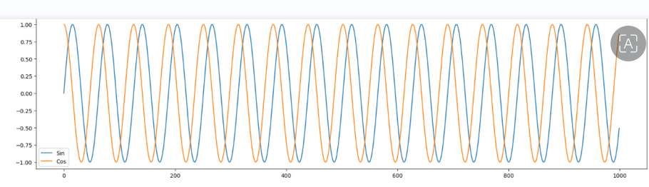
Each Data point is of format [sin,cos] . Sequence Length is 4 , so looking at past 4 datapoints we will predict the next datapoint in the sequence.

Setting up code

x = np.linspace(0,100,1000)
sin = np.sin(x)
cos = np.cos(x) 
plt.figure(figsize=(20,5))
plt.plot(sin, label = 'Sin')
plt.plot(cos, label = 'Cos')
plt.legend()

Our loss surface looks like this :

Data Plot 1

Setting up Dataset & DataLoaders

class TrignoDS(Dataset):
    def __init__(self,data):
        self.input_size = 2
        self.seq_length = 4
        X,Y = self.make_data(data)
        self.X = X
        self.Y = Y

    def make_data(self,data):
        x_tensor = torch.tensor([data[i:i+self.seq_length] for i in range(0, len(data) - self.seq_length)]).float()
        y_tensor = torch.tensor([data[i] for i in range(self.seq_length, len(data))]).float()
        return x_tensor,y_tensor

We prepare the data as described in problem statement. Please note that this is not complete ( please refer github link for complete reference)

Coding our RNN using pytorch

These are the equations governing how RNNs work 
h_t = f(Wx.X + Wh.Ht-1 + Bh )
y_t = g(Wy.Ht + By )

class RNN(nn.Module):
    def __init__(self,input_length , hidden_state_length , output_length):
        self.get_ht = nn.Linear(self.hidden_length+self.input_length,self.hidden_length)
        self.get_yt = nn.Linear(self.hidden_length+self.input_length,self.output_length)

    def forward(self,hiddens,inputs):
        data = torch.concat((hiddens,inputs),dim=1)
        ht = self.tanh(self.get_ht(data))
        yt = self.tanh(self.get_yt(data))
        return ht,yt

Note : only important parts of code are here

Function get_ht computes hidden state at time t & get_yt computes output at time t. If you look at the equation you will realise that h_t can be written as f( linear transformation of vector [X:H_t-1]) . Similarly y_t is a non linear transformation of H_t i.e. gof( linear transformation of vector [X:H_t-1]).

We can think of this as getting non linear transformation of linear transformation of input & past history content / state.

BTW, If you think something is incomplete in forward function ? You are absolutely right . Where is the logic for processing time steps ?

I am going to do it outside forward function & iterate over time in loop ( which we will see below ), however you can add the complete logic here as well.

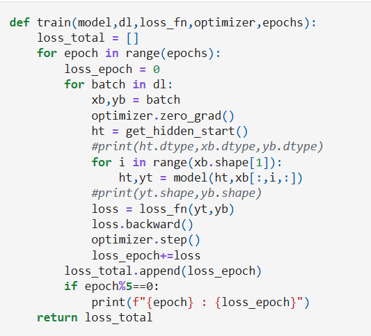
Setting up training loop

Here we are iterating over the sequence length to get the output from RNN . One reason for doing this was that it gives me freedom to decide what sort of architecture I want.

Here i wanted to only include loss from final step , however we could include loss from every step as well if the problem demands that ( ex NER ).

RNN traning loop

Summing it all together :

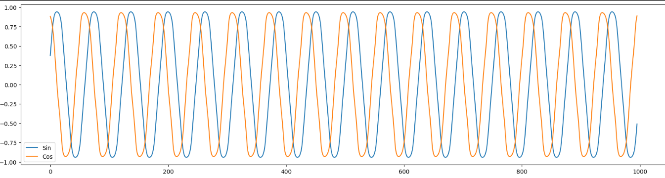
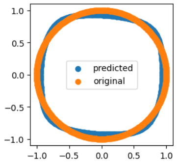
We get the following predictions for our sin & cos sequence : output 1 output 2

References:

https://karpathy.github.io/2015/05/21/rnn-effectiveness/

Tags: RNN

RNN

A Gentle Dive into implementing RNN using pytorch!