In this post we would implememt LSTM from scratch. To increase understanding I would use a small circular example dataset. Code implementation for this blog can be found in the github repo . This is related to the previous blog on RNN

Please Note that this blog will not dive deep into what an LSTM is or how it works. Better blogs than what I could write already exists. Scope of this blog is just implementing a vanilla LSTM using pytorch.

Setting up the problem statement

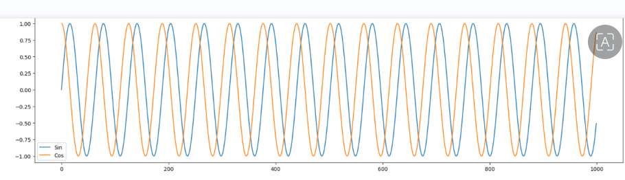
Each Data point is of format [sin,cos] . Sequence Length is 4 , so looking at past 4 datapoints we will predict the next datapoint in the sequence.

Setting up code

x = np.linspace(0,100,1000)
sin = np.sin(x)
cos = np.cos(x) 
plt.figure(figsize=(20,5))
plt.plot(sin, label = 'Sin')
plt.plot(cos, label = 'Cos')
plt.legend()

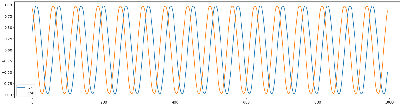
Our loss surface looks like this :

Data Plot 1

Setting up Dataset & DataLoaders

class TrignoDS(Dataset):
    def __init__(self,data):
        self.input_size = 2
        self.seq_length = 4
        X,Y = self.make_data(data)
        self.X = X
        self.Y = Y

    def make_data(self,data):
        x_tensor = torch.tensor([data[i:i+self.seq_length] for i in range(0, len(data) - self.seq_length)]).float()
        y_tensor = torch.tensor([data[i] for i in range(self.seq_length, len(data))]).float()
        return x_tensor,y_tensor

We prepare the data as described in problem statement. Please note that this is not complete ( please refer github link for complete reference)

Coding our LSTM using pytorch

\[f_t = \sigma(W_f \ x_t + U_f \ h_{t-1} + b_f) \\ i_t = \sigma(W_i \ x_t + U_i \ h_{t-1} + b_i) \\ \tilde{c}_t = \tanh \ (W_g \ x_t + U_g \ h_{t-1} + b_g) \\ c_t = f_t \circ c_{t-1} + i_t \circ \tilde{c}_t \\ o_t = \sigma(W_o \ x_t + U_o \ h_{t-1} + b_o) \\ h_t = o_t \circ \tanh \ (c_t)\]

f_t : How much of long term context to remember

i_t : How much of new candidate context to remember

$\tilde{c}_t$ : candidate context

c_t : context at time t

o_t : How much of long term context to expose

h_t : hidden short term context at time & the exposed state

These are the equations governing how LSTM works 


class LSTM(nn.Module):
    def __init__(self,input_length , hidden_state_length , output_length):
        super().__init__()
        self.hidden_length = hidden_state_length
        self.output_length = output_length
        self.input_length = input_length
        self.get_ft = nn.Linear(self.hidden_length+self.input_length,self.hidden_length)
        self.get_it = nn.Linear(self.hidden_length+self.input_length,self.output_length)
        self.get_ct = nn.Linear(self.hidden_length+self.input_length,self.output_length)
        self.get_ot = nn.Linear(self.hidden_length+self.input_length,self.output_length)      
        self.tanh = nn.Tanh()
        self.sigmoid = nn.Sigmoid()
    def forward(self,context,hiddens,inputs):
        data = torch.concat((hiddens,inputs),dim=1)
        ft = self.sigmoid(self.get_ft(data))
        it = self.sigmoid(self.get_it(data))
        ot = self.sigmoid(self.get_ot(data))
        candidate = self.tanh(self.get_ct(data))
        ct = ft*context + it*candidate
        ht = self.tanh(ct)*ot
        return ht,ct

Note : only important parts of code are here

So I had a few questions when looking at the architecture of an LSTM :

1. Why not just use ct , why even introduce ht if ht is a transformation of ct ?

cₜ is the “core memory,” and hₜ (the hidden state) is a filtered, non-linearly transformed view of it. ct is not bounded (it can grow large), and it accumulates information over time. Using tanh(cₜ) bounds it to [-1, 1], making it more stable to expose to downstream layers.

2. Why tanh & sigmoid , why not sigmoid everywhere ? why not Relu ?

Sigmoid is used as a transformation to get probability of the signal ( gated output ) . Tanh is used as negative signals need to be captured . Relu / sigmoid will scrap the negative signals all together

3. Why not connect f_t & i_t ?

Turns out thats one of the things a GRU optimizes

4. Forget gate , input gate ? ..aaaah headache

So we can just remember one thing , there is a long term context ct which is calculated as weighted sum of last context & current possible context . This is then non linearly transformed into short term memory a.k.a hidden state a.k.a exposed state i.e. h_t

Summing it all together :

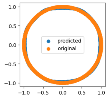
We get the following predictions for our sin & cos sequence : output 1 output 2

References:

https://karpathy.github.io/2015/05/21/rnn-effectiveness/

https://colah.github.io/posts/2015-08-Understanding-LSTMs/

Tags: RNN LSTM

LSTM

A Gentle Dive into implementing LSTM using pytorch!